In Lectures 5, we have introduced the concept of conditional probability and see how we could use it to learn from the real world. Whenever we come across a new concept, the first thing is always to build up our intuition about it. Using a few simple examples, we start to get some ideas about conditional probabilities.
In conditional probability, we are interested in calculating the probability of an event when taking into account some knowledge that we have. Recall that $\mathbb{P}(A)$ denotes the probability of event $A$, which represents our belief on how likely event $A$ will occur. Now we know another event $B$ has occurred. Taking this new piece of information into account, what is the probability of event $A$ to occur? That is basically the probability of $A$ given $B$, denoted by:
$$\mathbb{P}(A|B)$$
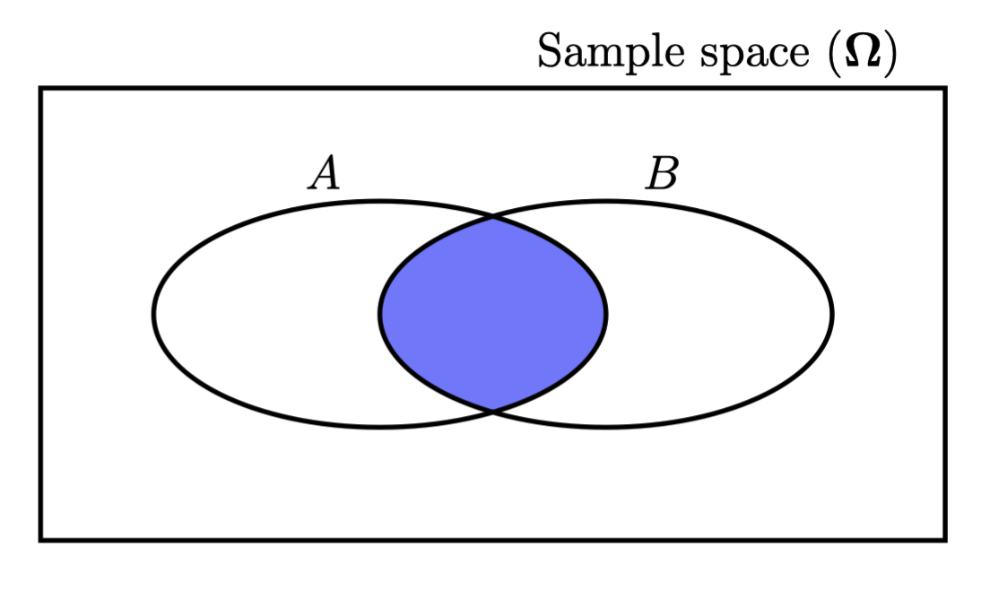
We could look at the following Venn diagram:

Before we know anything or have any information, we think the probability of $A$ to occur is $\mathbb{P}(A)$, which can be treated as the ratio of the areas between the ellipse $A$ and the rectangle. When we know that $B$ has occurred, all of a sudden we are living in a universe where $B$ has already occurred. That’s is a fact now, and everything outside the ellipse $B$ becomes irrelevant. Our new sample space becomes $B$. Now we ask what is the probability of $A$, that is, $\mathbb{P}(A|B)$. In this case, it is the ratio of the blue area and the ellipse $B$. Therefore, it is straightforward to see:
$$\mathbb{P}(A|B)=\cfrac{\mathbb{P}(A \cap B)}{\mathbb{P}(B)} \textmd{, } \mathbb{P}(B) \neq 0$$
You see, there are three different probabilities in the above equation: $\mathbb{P}(A \cap B)$, $\mathbb{P}(B)$ and $\mathbb{P}(A|B)$. We are going to introduce how to calculate each of them. In addition, the new probability $\mathbb{P}(A|B)$ may or may not be the same as $\mathbb{P}(A)$, value-wise. We will see why we care about it in future.
When dealing with the conditional probability, remember that it is just normal probability in a new universe or a different (often smaller) sample space. For those properties we have in the normal probability, we also have them in the conditional probability. For example, for all the probability axioms, we have a conditional version of each of them:
- Nonnegativity: $\mathbb{P}(A|C) \geqslant 0$, for every event $A$
- Normalisation: $\mathbb{P}(\Omega|C) = 1$
- Additivity: If $A$ and $B$ are disjoint given $C$ has occurred ($A \cap B|C = \varnothing$), then: $$\mathbb{P}(A \cup B | C) = \mathbb{P}(A|C) + \mathbb{P}(B|C)$$
During the lecture we used the “virus detection” example to showcase how sometimes conditional probabilities can provide counterintuitive results. However, if we adjust our way of thinking, we will see that the results not only make sense, but help us approach real-life problems in a more rational way as well.