Now we have get familiar with conditional probabilities. The basic definition and formula is:
$$\mathbb{P}(A|B)=\cfrac{\mathbb{P}(A \cap B)}{\mathbb{P}(B)} \textmd{, } \mathbb{P}(B) \neq 0$$
In the previous lecture, we used some examples to show how to calculate three probabilities: $\mathbb{P}(A \cap B)$, $\mathbb{P}(B)$ and $\mathbb{P}(A|B)$, which are essentially the three terms in the above formula. In reality, we sometimes need to calculate some very complicated probabilities, but they all boils down to some sort of combinations of those three probabilities. Therefore, let’s generalise those calculations and make them more useful.
We introduce three basic rules: the multiplication rule for calculating $\mathbb{P}(A \cap B)$ or the like, the total probability rule for $\mathbb{P}(B)$ or the like, and the Bayes’ rule for $\mathbb{P}(A|B)$ or the like.
The Multiplication Rule
$$\mathbb{P} ( \cap_{i=1}^n A_i ) = \mathbb{P}(A_1)\mathbb{P}(A_2|A_1)\mathbb{P}(A_3|A_1 \cap A_2) \cdots \mathbb{P} ( A_n | \cap_{i=1}^n A_i )$$
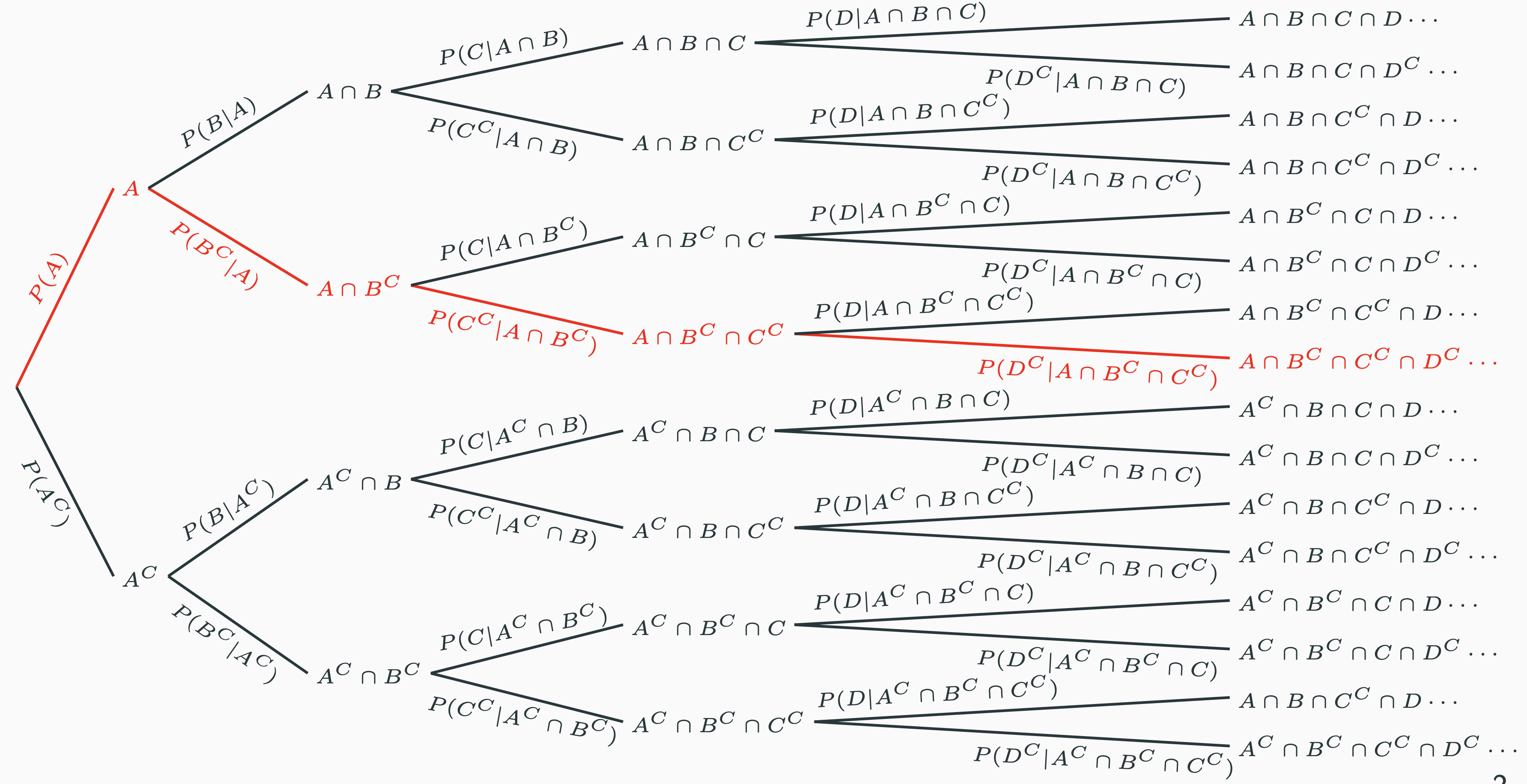
When a complicated event can be written as the intersection of a sequence of events, the probability can be calculated using the multiplication rule. You do not have to memorise the equation at all. Instead, you could put the following picture in your mind:

We build a tree with the root at the left, which is our starting point. The event of our interest is basically a leaf, which can be divided into a sequence of events along the path starting from the root. The probability on each branch is the conditional probability conditioned on the previous leaf. In this way, the probability of any event of interest can be calculated by traversing the branches and multiplying all the probabilities along the path from the root to that leaf. That is essentially what the multiplication rule tells us.
For example, in the above picture we want to calculate $\mathbb{P}(A \cap B^C \cap C^C \cap D^C)$. We first locate the leaf $A \cap B^C \cap C^C \cap D^C$. Then we identify the path from the root to that leaf, i.e. the red path. In this path, we encountered $\mathbb{P}(A)$, $\mathbb{P}(B^C|A)$, $\mathbb{P}(C^C|A \cap B^C)$ and $\mathbb{P}(D^C| A \cap B^C \cap D^C)$ sequentially along the way. Therefore, we simply multiply them altogether:
$$ \mathbb{P}(A \cap B^C \cap C^C \cap D^C) = \mathbb{P}(A) \cdot \mathbb{P}(B^C|A) \cdot \mathbb{P}(C^C|A \cap B^C) \cdot \mathbb{P}(D^C| A \cap B^C \cap D^C) $$
The Total Probability Rule
$$\mathbb{P}(B) = \sum_{i=1}^{n}\mathbb{P}(A_i)\mathbb{P}(B|A_i)$$
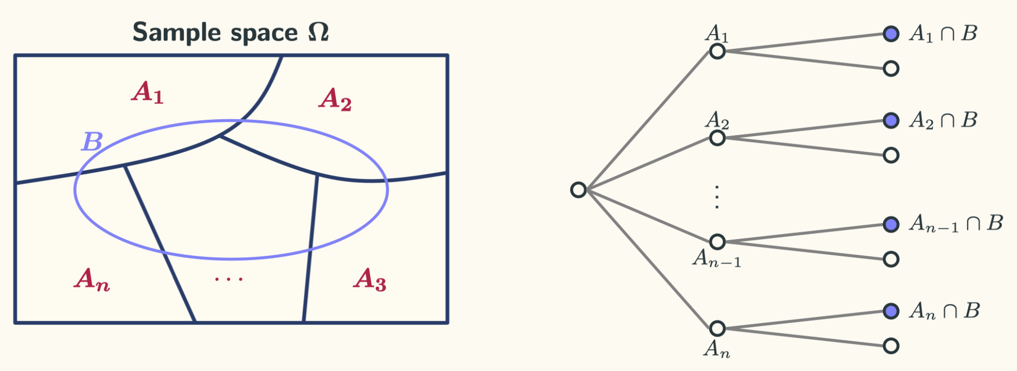
This can be viewed as the weighted average of the conditional probability $\mathbb{P}(B|A_i)$, with the original probability $\mathbb{P}(A_i)$ as the weight. Again, you do not have to memorise this equation. Instead, put the following two figures in your mind:

The two figures tell us essentially the same thing. The left figure tells us that to calculate the probability of an event $B$, we could use a “divide-and-conquer” strategy. We divide our event of interest $B$ into a sequence of disjoint events. Then the total probability of $B$ is basically the sum of the probability of each of the sub-event according to the additivity axiom. The right figure shows an equivalent sequential model. Event $B$ can be divided into a sequence of leaves. The total probability of $B$ can be calculated using the sum of each leaf. How do we calculate the probability of each leaf then? Well … just use the multiplication rule.
I think the two figures above more intuitive than the formula itself. Both figures are useful under different circumstances.
The Bayes’ Rule
$$\mathbb{P}(A_i|B) = \cfrac{\mathbb{P}(A_i)\mathbb{P}(B|A_i)}{\sum_{i=1}^n \mathbb{P}(A_i)\mathbb{P}(B|A_i)}$$
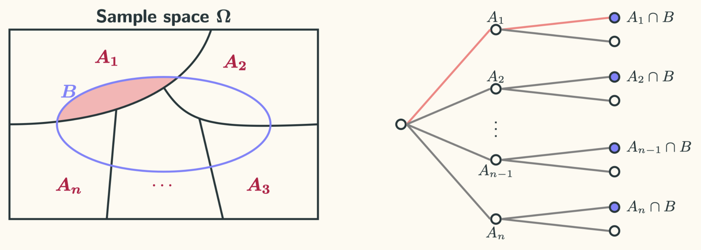
The Bayes’ rule is often used for inference. We often learn new information from the real world, and we use the new information to update our prior belief. The Bayes’ rule shows us how we should do that in a systematic way. We think there is some causal effect from $A_i$ to $B$, modelled by the probability $\mathbb{P}(B|A_i)$. Once we observe that $B$ has occurred, we want to say something about (inference) $A_i$, which is modelled by the probability $\mathbb{P}(A_i|B)$. Again, DO NOT simply memorise the equation. You will find yourself confused when seeing a different version of it, especially when the order of $A$ and $B$ is swapped in some text books. Instead, put the following figures in your mind (similar to the previous ones):

What those pictures tell us is that we have a sequence of disjoint events $A_i$, and each of them has a certain probability to happen. Under each of them, $B$ may or may not happen. Now we have observed that $B$ has occurred. What can we say about $A_i$? This is essentially what we were doing during the lectures. Perhaps we could re-write the equation in a slightly different way:
$$\mathbb{P}(A_i|B) = \cfrac{\mathbb{P}(B|A_i)}{\mathbb{P}(B)} \cdot \mathbb{P}(A_i)$$
When we do not have any information, we have certain belief about how likely $A_i$ might happen. That is basically $\mathbb{P}(A_i)$, which is called the prior probability. Once we have some new knowledge, that is, we observe that $B$ has occurred. We use that piece of new information to update our belief about how likely we think $A_i$ will occur. That is basically $\mathbb{P}(A_i|B)$, which is called the posterior probability. It shows us we could learn new things from the real world, and we could do this systematically by multiplying the prior probability by a coefficient.
Therefore, when analysing a real life problem, always ask yourself first: what is the probability of the event of interest before you see any new information. Then, once some new information is provided, do you change your original belief about the event? That is the basic idea and intuition of the Bayes’ theorem.