Lecture 20 Confidence Interval For The Variance

Once we have introduced the confidence intervals for the population mean $\mu$, the next question comes natural: how do we construct confidence intervals for the population variance $\sigma^2$? Since we have previously discussed the sampling distribution of the sample variance, it is kind of straightforward for us to derive the confidence interval for the population variance.

Interval Estimation For $\boldsymbol{\sigma^2}$

We can just follow the same thought from the previous lecture when we derived the CI for the population mean $\mu$. Let’s start with what we know about the variance. If you recall, we know that:

$$\cfrac{(n-1)S^2}{\sigma^2} \sim \chi^2(n-1)$$

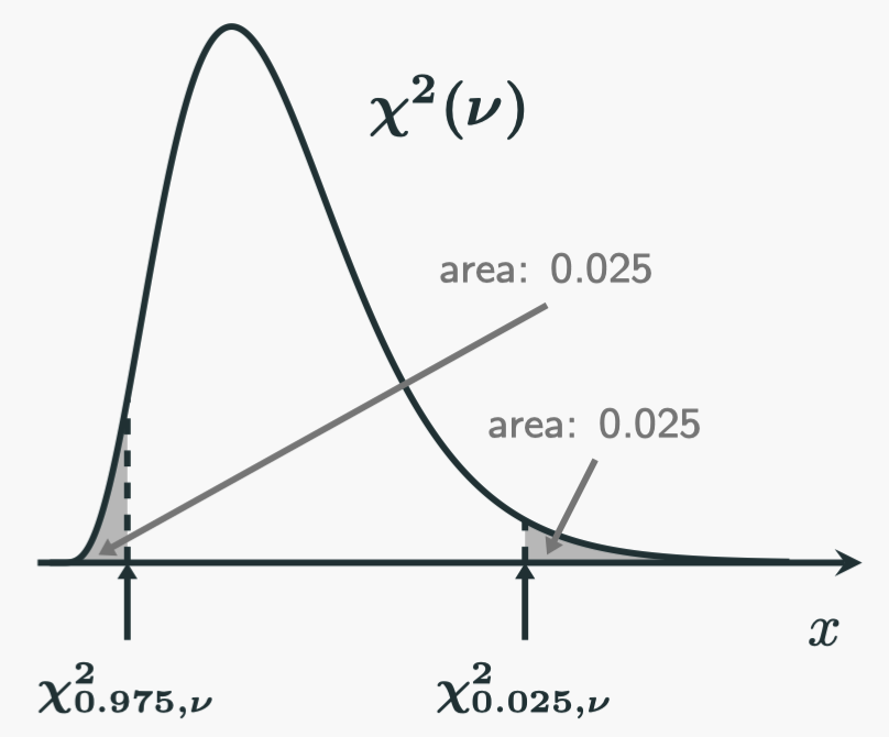
Since the $\chi^2$-distribution has a well defined PDF, we could use it to help us to calculate probabilities. If we want a two-sided 95% CI for $\sigma$, we often would like a “symmetrical” one. We can put the following picture in our head to help us visualise in the same way when we construct the CI for the mean:

The probability of a $\chi^2$ random variable with a degree of freedom $\nu$ falling into the middle white area is $95\%$. Therefore, we start from there (note all of them are positive numbers):

$$ \begin{aligned} \mathbb{P} \left( \chi^2_{0.975,n-1} \leqslant \chi^2 \leqslant \chi^2_{0.025,n-1} \right) &= 0.95\\[10pt] \mathbb{P} \left[ \chi^2_{0.975,n-1} \leqslant \cfrac{(n-1)S^2}{\sigma^2} \leqslant \chi^2_{0.025,n-1} \right] &= 0.95\\[10pt] \mathbb{P} \left[ \cfrac{1}{\chi^2_{0.025,n-1}} \leqslant \cfrac{\sigma^2}{(n-1)S^2} \leqslant \cfrac{1}{\chi^2_{0.975,n-1}} \right] &= 0.95\\[12.5pt] \mathbb{P} \left[ \cfrac{(n-1)S^2}{\chi^2_{0.025,n-1}} \leqslant \sigma^2 \leqslant \cfrac{(n-1)S^2}{\chi^2_{0.975,n-1}} \right] &= 0.95 \end{aligned} $$

Now we have get our 95% CI for the population variance $\sigma^2$:

$$\left[ \cfrac{(n-1)S^2}{\chi^2_{0.025,n-1}}, \cfrac{(n-1)S^2}{\chi^2_{0.975,n-1}} \right]$$

Whenever we have a sample, the values of $S$ and $n$ are determined. We could put the numbers in to get the 95% CI.

Conditions To Use The Technique

Now we summarise below the confidence intervals we have constructed so far. The two-sided confidence intervals with $(1-\alpha) \times 100\%$ confidence level are:

One thing we need to remember is that when we construct those CIs, there are some assumptions. Therefore, there are conditions for us when we use the above formulae. Let’s look at them explicitly.

First of all, we need the sample $X_1,X_2,\cdots,X_{n-1},X_n$ to be i.i.d.. Therefore, the sample must be randomly and independently selected from the population. If this is not the case, the sample is not a good representation of the population, so the conclusion will not be useful. This condition must be met for all statistical inferences besides confidence intervals.

Now let’s look at those CIs one by one. The reason we use $\bar{X} \pm Z_{\frac{\alpha}{2}} \cdot \frac{\sigma}{\sqrt{n}}$ is predicated on the assumption that

$$\cfrac{\bar{X} - \mu}{\sigma/\sqrt{n}} \sim \mathcal{N}(0,1)$$

When is that true? It is true when $\bar{X}$ follows a normal distribution. When does $\bar{X}$ follow a normal distribution? When the population is normally distributed or the sample size is large enough.

Further, the reason we use $\bar{X} \pm t_{\frac{\alpha}{2},n-1} \cdot \frac{S}{\sqrt{n}}$ is predicated on the assumption that

$$\cfrac{\bar{X} - \mu}{S/\sqrt{n}} = \cfrac{\frac{\bar{X}-\mu}{\sigma/\sqrt{n}}}{\sqrt{\frac{(n-1)S^2}{\sigma^2} \cdot \frac{1}{n-1}}} \sim \boldsymbol{\mathcal{T}}(n-1)$$

When is that true? When the numerator $\frac{\bar{X} - \mu}{\sigma/\sqrt{n}}$ follows a standard normal distribution AND the term $\frac{(n-1)S^2}{\sigma^2}$ in the denominator follows a $\chi^2(n-1)$ distribution. When are those true? We already talked about the numerator. For $\frac{(n-1)S^2}{\sigma^2}$ to follow a $\chi^2(n-1)$ distribution, we need the population to be normally distributed.

Similarly, the reason we use $\left[ \cfrac{(n-1)S^2}{\chi^2_{\frac{\alpha}{2},n-1}}, \cfrac{(n-1)S^2}{\chi^2_{1-\frac{\alpha}{2},n-1}} \right]$ is predicated on the assumption that

$$\cfrac{(n-1)S^2}{\sigma^2} \sim \chi^2(n-1)$$

That is true when the population to be normally distributed.

As you can see, in order to use the formulae in the table to construct CIs, we need the following assumptions to be true:

1. The samples are randomly and independently selected from the population
2. The normality condition: The population is normally distributed.
3. When $\sigma$ is known, and we want a CI for the mean $\mu$, as long as the sample size is large enough, it is still okay even if the population is not normally distributed.

The point I want to make here is to showcase that those assumptions all come natural if you truly understand the principles.

Violation of The Normality Assumption

We can use some simulations to see what happens when we draw sample from a non-normal distribution. I use some python code for the demonstration, and just use the distribution of the sample variance as an example. You can try others by yourself.

Let’s start with a heavily skewed distribution, such as an exponential distribution:

# import some helper functions from common libraries
import numpy as np
from scipy.stats import norm, chi2, poisson, expon
import matplotlib.pyplot as plt

# create an exponential population with a rate parameter 1
pop_expo = expon(scale = 1)
pop_var = pop_expo.var() # population var is 1

# we can have a look at the shape of the population distribution
# you can see it is heavily skewed to the right by uncommenting the next line
# plt.plot(np.linspace(0,10,100), pop_expo.pdf(np.linspace(0,10,100)))

# now we draw a sample with size n=10
# each time we draw a sample, we compute the score (chiscore) and record it
# we repeat the process 10,000 times
# so we have 10,000 chiscore
n = 10          # sample size
chiscores = []  # place holder for chiscore in each sample

for _ in range(10000):
    sample = pop_expo.rvs(size = n)       # draw a sample with size n
    s2 = sample.var(ddof = 1)          # compute the sample variance
    chiscore = (n - 1) * s2 / pop_var  # compute the chiscore
    chiscores.append(chiscore)         # record the chiscore

# now we can compare the distribution of chiscores with
# a theoretical chi-squared distribution with n-1 DOF
rv = chi2(n-1)   # create a chi-squared random variable with n-1 DOF

### look at the histogram of the chiscores from the simulation in red colour
plt.hist(chiscores, bins = 50, density = True, color='r', ec='k') 
### look at the theoretical density function of a chi-squared rv with n-1 DOF in blue colour
plt.plot(np.linspace(0, n*5, 100), rv.pdf(np.linspace(0, n*5, 100)), 'b-')
plt.show()

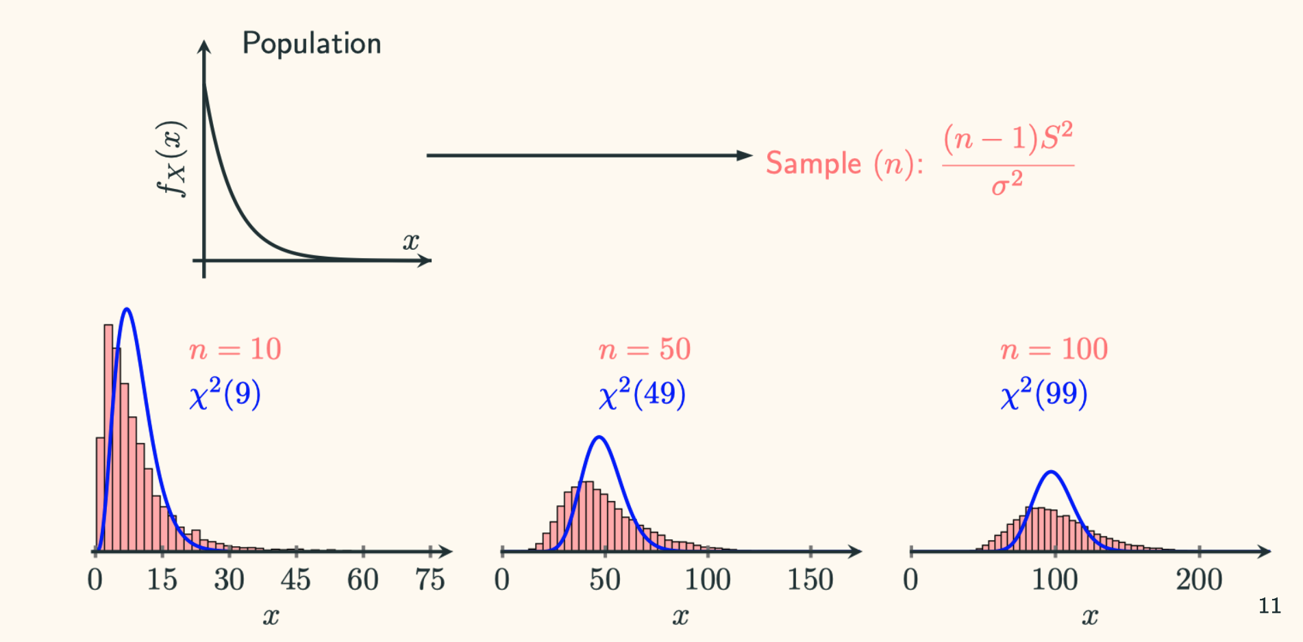
You can manipulate the above code to check different sample size. I have tried $n=10,50,100$. The results are shown below:

As you can see, they do not really fit even with large sample sizes.

We can also manipulate the above code to see what happens from a different kind of population. Say, we draw samples from a Poisson population with a mean $\lambda = 4$. This is achieved by:

pop_pois = poisson(4)
pop_var = pop_pois.var() # population variance is 4

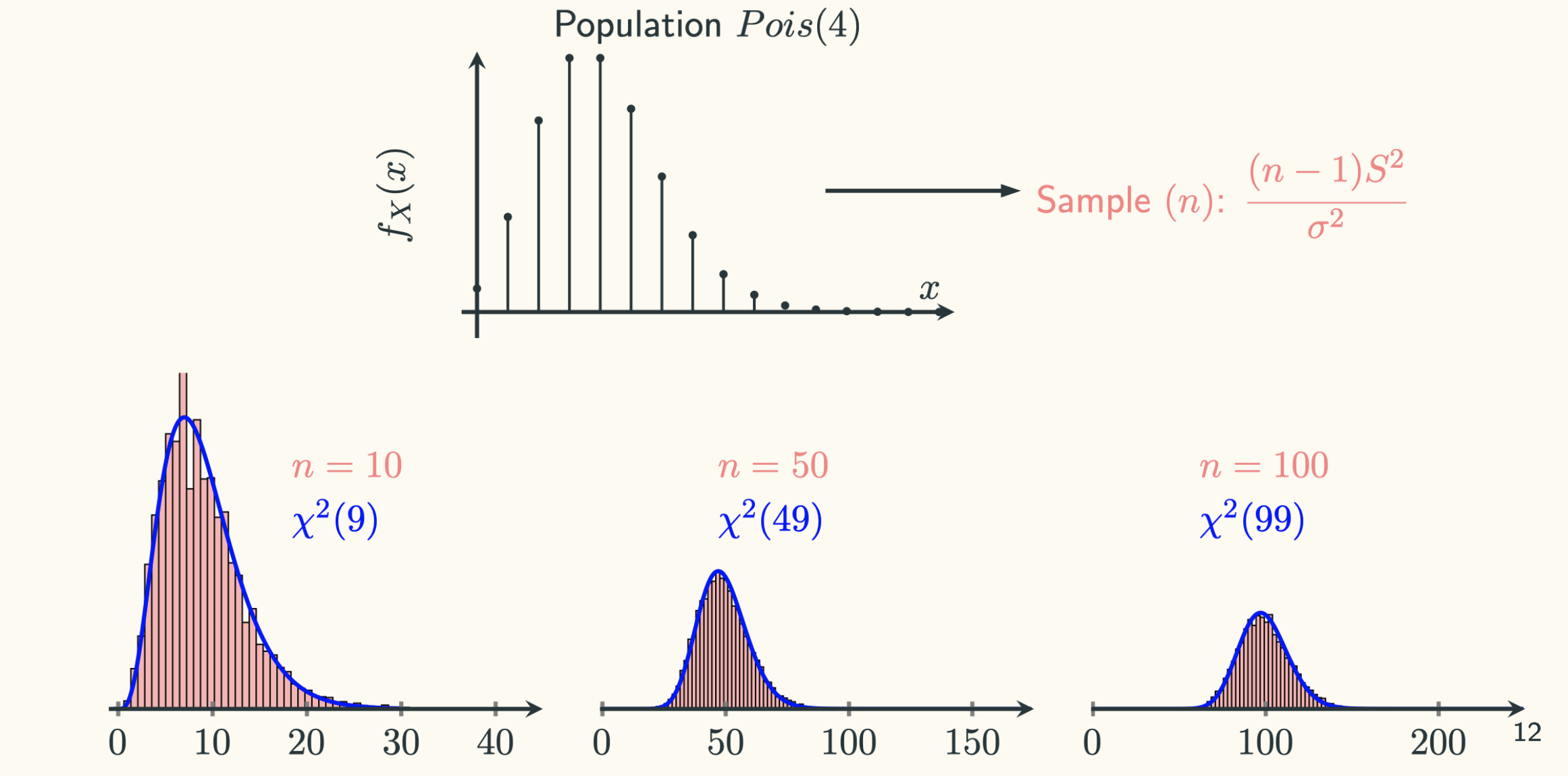
The simulation results are:

In this case, it is not bad at all, even $Pois(4)$ is not normal. Notice that $Pois(4)$ is roughly symmetrical around its mean. Even though the population is still skewed to the right, but the data after $x > 10$ is negligible.

Therefore, in practice, it is not the end of the world when the “normality” condition is violated, especially when the population is roughly symmetrical.