Lecture 22 Confidence Interval For The Proportion

Now that we have figured out the sampling distribution of the sample proportion, we can make interval estimation and construct confidence intervals for the sample proportion. Before we do that, let’s use an example to look the distribution of $P$ one more time.

A Simplified Version of Gene Expression

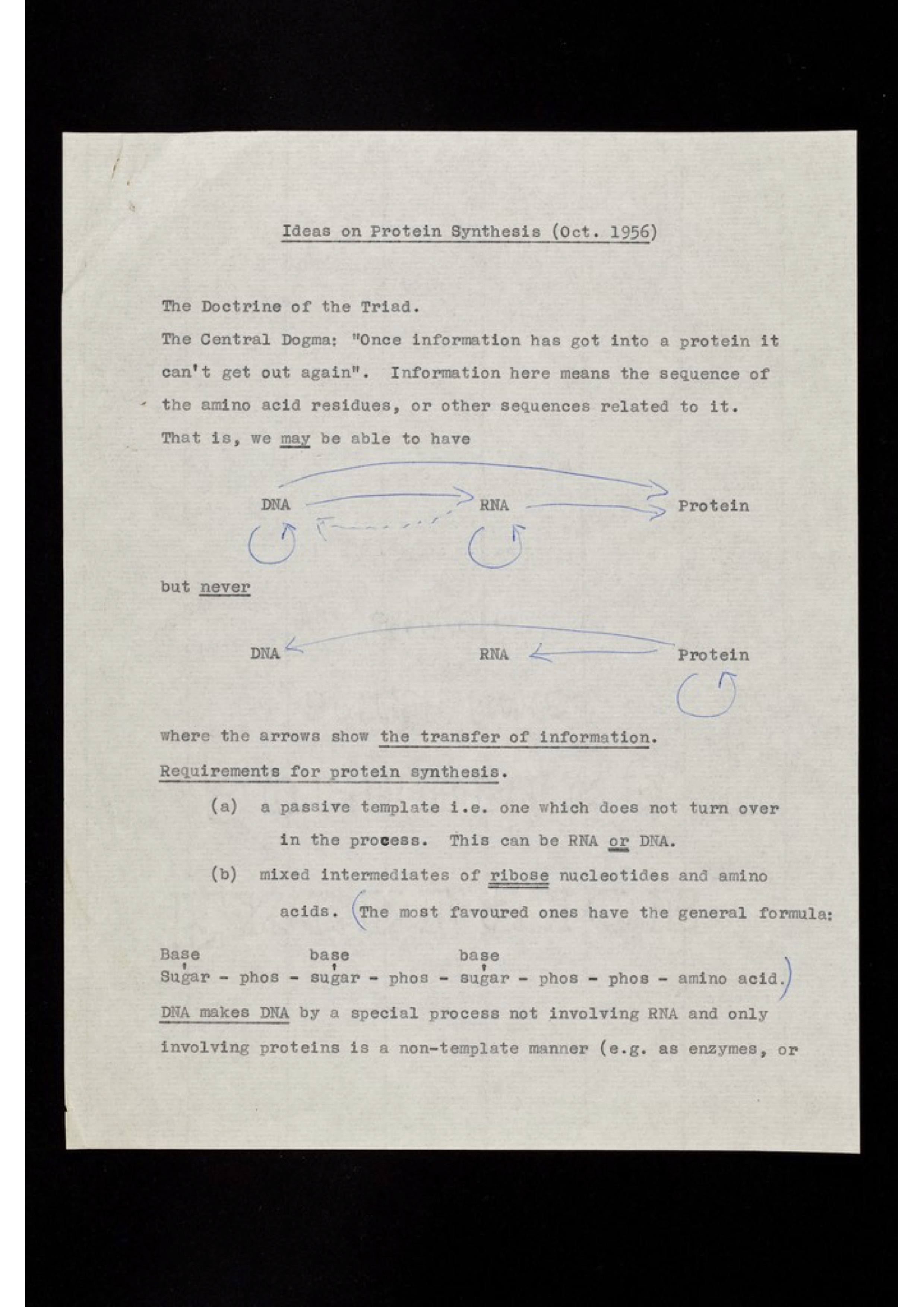
As we know, DNA is our genetic material. In order for a gene to function, the gene needs to be “converted” into proteins¹. This process is describe by the central dogma of molecular biology that we learnt in high school. Here is the draft version of it from Francis Crick’s conference notes in a symposium held at London back in 1957, one year before the central dogma was officially published:

Credit: “Ideas on protein synthesis (Oct. 1956)”. Wellcome Collection. In copyright

The first step is the conversion into RNA using DNA as the template, a procedure called transcription. In modern days, we have sequencing technologies to quantify the number of RNA molecules of each gene in a particular sample (see Lecture 1). Getting those numbers is very important, because they can tell us many things about the sample we study, such as the status and the identity. Different genes may have different numbers of RNA molecules in a sample. For example, the gene GAPDH encodes an enzyme that is important for glycolysis. The cells need a lot of it, so it has many RNA molecules to be translated into proteins. Other genes may not have that many RNA molecules, not because they are not important,but for many complicated reasons which are left for you to explore in your molecular and cell biology class.

There are over 20,000 genes. Each time we perform an experiment, we get certain number of molecules from a sample. Those molecules basically come from those 20,000 genes, so we have 20,000 integer values for each experiment, representing molecular counts for those genes. However, experiments are ever perfect. We never get the same amount of molecules even for the same sample. Let’s say, we have three different experiments. In the first one, we are able to obtain 20 million molecules; in the second experiment, we capture 40 million molecules and the third 30 million molecules. Once we are done, we observe that the number of molecules of GAPDH in those three experiments are $1990$, $4020$ and $3005$, respectively. Can we say that the true values of GAPDH in those three experiments are different? Probably not. The differences might be caused by the total number of molecules we get per experiment. Remember the total number of molecules are the results of 20,000 genes. Therefore, it is the relative quantity of the RNA of the gene that is of our interest, that is, the sample proportion we talked about. We call it the gene expression level.

Now let’s see a different gene called PLK1, which is an essential genes for the cell cycle progression. Its gene expression level is not as high as GAPDH, and say we know its true gene expression level as:

$$\pi = 0.000001126088083$$

Let’s think about this number for a moment before we move on. This might look like a really really tiny fraction, but if you think about it a bit more, it actually makes sense. When we talk about the proportion in terms of the fraction or the percentage, the total sum is $1$ or $100%$, respectively. That comes from over 20,000 genes, so eventually each gene only takes a very small fraction or percentage of the total. To make that number look a bit prettier, we do not talk about percentage (per $\boldsymbol{100}$) when dealing with gene expression levels. We use per million ($\boldsymbol{10^6}$), which is still just a proportion at a different scale.

Now we ask the following question: what is the sampling distribution of the sample proportion of PLK1 if we draw one million $(10^6)$ molecules from the population? We use what we learnt in the last lecture and expect the proportion should follow:

$$P_{PLK1} \ \dot\sim \ \mathcal{N} \left(\mu_{P} = \pi = 1.126 \times 10^{-6}, \sigma_{P}^2 = \cfrac{\pi(1-\pi)}{n} = 1.126 \times 10^{-12} \right)$$

We can do some simulations on the computer to see if our expectation is correct. The following is some very crude python codes for this purpose, but it works and the speed is acceptable:

# import some helper modules
import numpy as np
from collections import Counter

# set the seed
np.random.seed(42)

# the expression level of PLK1 is 0.000001126088083
# which is roughly 100 per 88803000
# so we create a array with 88802900 zeroes and 100 ones
molecules = np.zeros((88803000,))
molecules[:100] = 1

# then we take 1000000 molecules from that
# check how many 1s (PLK1 molecules) there
# record the number
# repeat for 1000 times
results = [] # hold the number of PLK1 per experiment
## the following loop takes a few seconds
for _ in range(1000):
    plk1 = np.random.choice(molecules, 1000000).sum() # take 1e6 molecules, check how many 1s (PLK1)
    results.append(plk1)                              # record the number

# now look at the results
Counter(results)

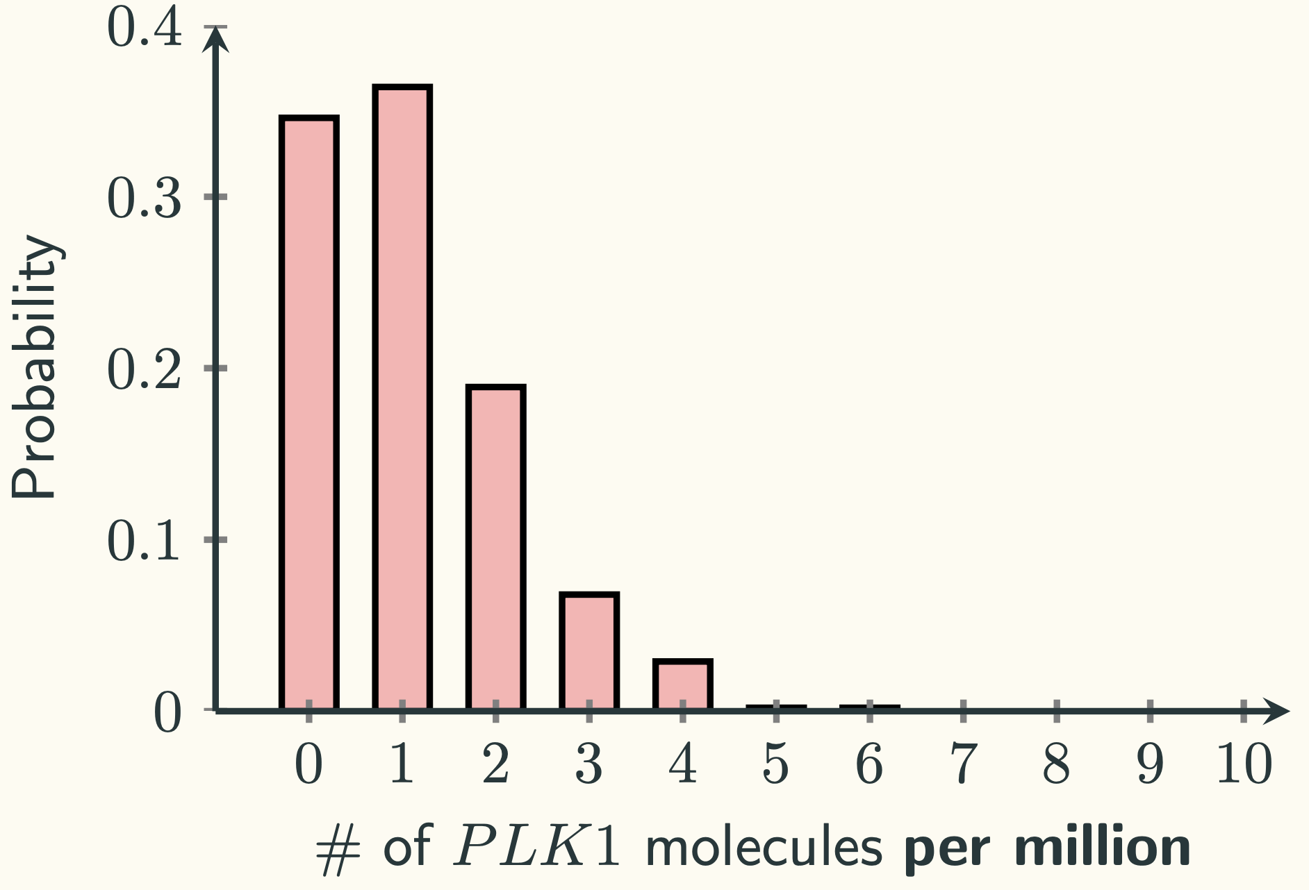
If you plot the results as PMF, you will see:

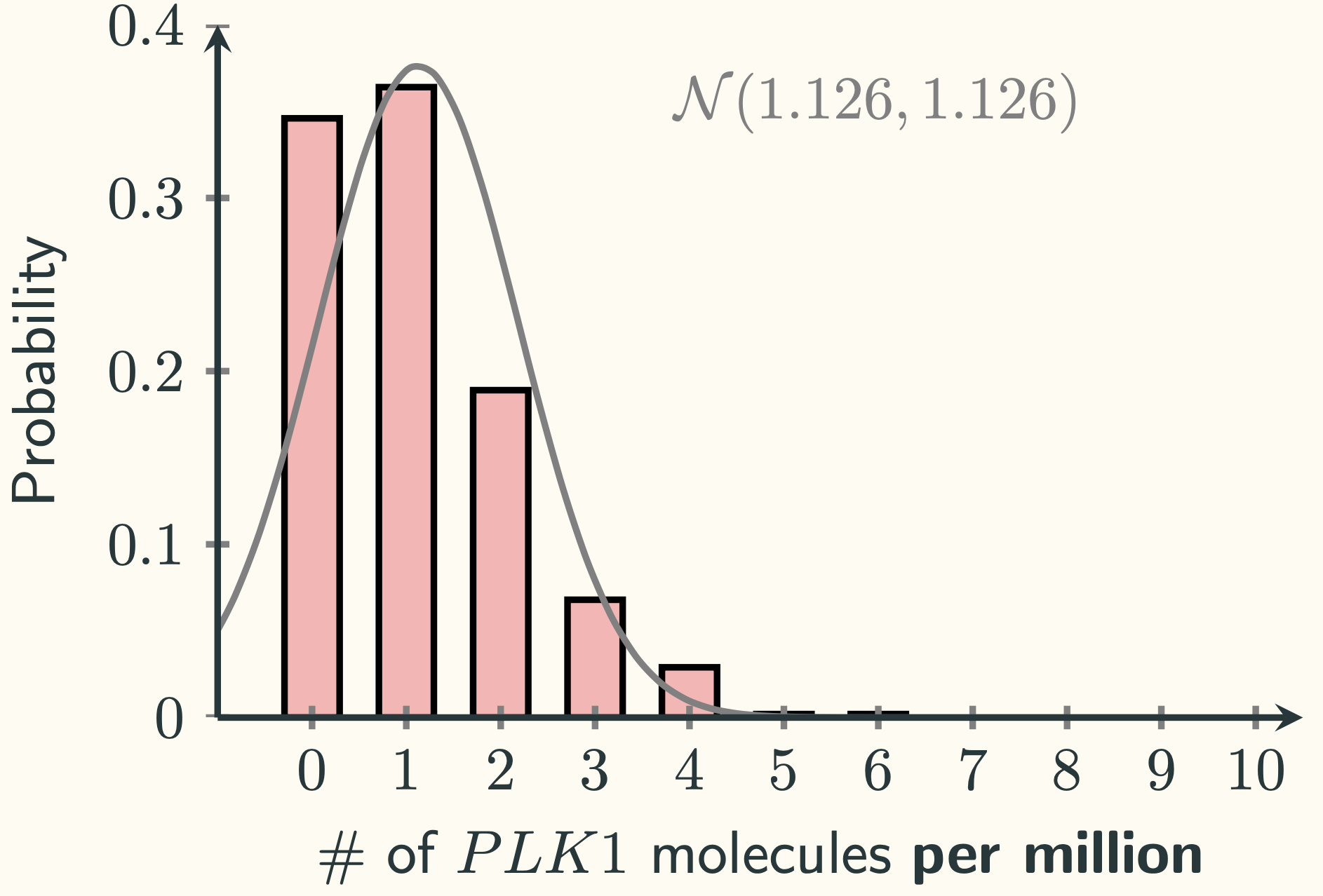
That looks like a positively skewed distribution. It will probably not be approximated by a normal distribution well, since normal distributions are symmetrical. Indeed, if we plot the normal distribution $\mathcal{N}\left(1.126 \textmd{ per million}, 1.126 \textmd{ per million}^2\right)$ on top of it, we can see:

There are two things that we noticed from the above picture. The first one is that the centre of the gravity of the simulation data (red bars) lies between $0$ and $1$, but the theoretical normal distribution (the grey line) is centred on $1.126$. The second thing is that the simulation data does not take the negative values, but there is still a lot of data in the normal distribution at the negative side of the axis.

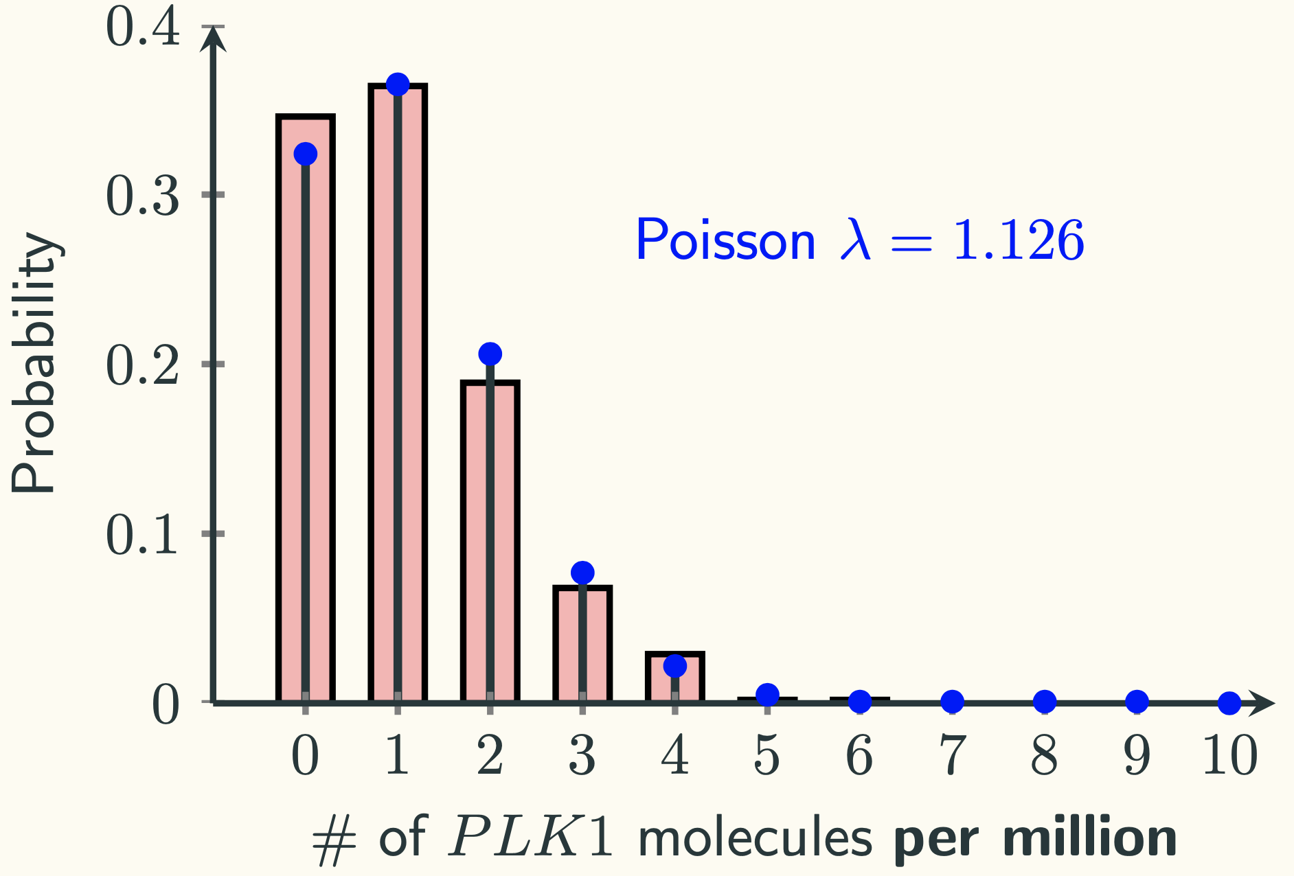
The red bars look a lot like a Poisson distribution. Indeed, if we put on top of a Poisson PMF with $\lambda = 1.126 \textmd{ per million}$, we have:

Conditions of The Normal Approximation

We were told that as long as the sample size is large enough, the sample proportion (the sample mean of the indicator variables) should follows a normal distribution, regardless of the distribution of the original population. Any reasonable person would think 1 million should be a sample size that is large enough. However, it seems the normal distribution does not work here. So what is going on here?

As we discussed in the last lecture, the distribution of the PLK1 gene expression in our experiment is essentially a binomial distribution with a really big $n$ and a really tiny $p$. It turns out that when the product of $n \cdot p$ small, the binomial is well approximated by a Poisson distribution with $\lambda = np$. When $n \cdot p$ is not small, the binomial can be approximated by a normal distribution with $\mu=np$ and $\sigma^2=npq$, where $q=1-p$.

I think it is relatively intuitive to understand the Poisson approximation. Recall how do we get the poisson PMF from Lecture 11. We let $p = \cfrac{\lambda}{n}$ and make $n$ goes to infinity, we get:

$$ \begin{aligned} & \lim_{n \to \infty} \binom{n}{k}\left( \cfrac{\lambda}{n} \right)^k \left(1-\cfrac{\lambda}{n} \right)^{n-k} \\[10pt] &= \cfrac{\lambda^k}{k!} \lim_{n \to \infty} \cfrac{n(n-1)\cdots(n-k+1)}{n^k} \cdot \left(1-\cfrac{\lambda}{n} \right)^n \cdot \left(1-\cfrac{\lambda}{n} \right)^{-\lambda} \\[10pt] &= \cfrac{\lambda^k}{k!} \cdot \left( 1 \cdot 1 \cdot e^{-\lambda} \right) \end{aligned} $$

The bigger $n$ is and the smaller $p = \cfrac{\lambda}{n}$ is, the better the approximation. One question that still remains is: why does the central limit theorem failed here?

Recall from Lecture 15 when we introduced the central limit theorem, we discussed “how large is large enough” in terms of sample sizes. It actually depends on the shape of the population distribution. When the population is normally distributed, $n=2$ is already large enough and its sampling distribution of the sample mean already follows a normal distribution. In our current situation, the population is heavily heavily skewed, with a $Ber(0.000001126088083)$. In this case, even 1 million is not large enough. Therefore, when dealing with proportions, “large enough” means $np \geqslant 10$. However, remember that the concept of “success (1)” or “failure (0)” is arbitrary. We also need $nq \geqslant 10$ at the same time, where $q=1-p$.

Now another question arises: why $np \geqslant 10$ AND $nq \geqslant 10$? Why not 5, 15, 20? Well … different people might have different thresholds. Some say 5, some say 10 like us, some say 15. Here, I’m not able to provide a solid proof, but I can give a rough and intuitive reasoning.

From the above pictures, we see that one reason the normal distribution fails to approximate the binomial is that there is still a lot of data outside the interval $[0,n]$ where all data from the binomial is located. For a normal distribution, the data is located from $-\infty$ to $\infty$. From the empirical rule, we know that about $99.7\%$ of the data are located within the interval $[\mu-3\sigma, \mu+3\sigma]$. Intuitively, if this interval is contained within $[0,n]$, then we would not have the problem that a lot of the data in the normal distribution is outside the binomial’s data range. Therefore, intuitively, we need:

$$0 < \mu-3\sigma \textmd{ and } \mu+3\sigma < n$$

We can replace the normal parameters with the binomial ones, starting from the first inequality:

$$ \begin{aligned} 0 &< \mu-3\sigma \\ 0 &< np - 3\sqrt{npq} \\ np &> 3\sqrt{npq}\\ n^2p^2 &> 9npq \\ np &> 9q = 9(1-p) = 9 - 9p \end{aligned} $$

Since the maximum value of $9-9p$ is $9$, so we choose the threshold of $np \geqslant 10$. Now the second inequality:

$$ \begin{aligned} \mu+3\sigma &< n \\ np + 3\sqrt{npq} &< n \\ 3\sqrt{npq} &< n-np = n(1-p) = nq\\ 9npq &< n^2 q^2 \\ nq &> 9p = 9(1-q) = 9 - 9q \end{aligned} $$

Similarly, the maximum value of $9-9q$ is $9$, so we choose the threshold of $nq \geqslant 10$.

In summary, when $n$ is large AND $np \geqslant 10$ AND $nq \geqslant 10$, we can use the normal distribution to approximate the binomial. When $n$ is large but $np$ or $nq$ is between 0 and 10, we can use the Poisson distribution for the approximation.

The Wald Interval

Now let’s see how to construct the 95% confidence interval for the proportion. We use the same method as before, using the properties of the sampling distribution of the sample proportion:

$$ \begin{aligned} \mathbb{P}\left(-1.96 \leqslant Z \leqslant 1.96 \right) = 0.95\\ \mathbb{P}\left(-1.96 \leqslant \cfrac{P-\mu_P}{\sigma_P} \leqslant 1.96 \right) = 0.95\\ \mathbb{P}\left(-1.96 \leqslant \cfrac{P-\pi}{\sqrt{\frac{\pi(1-\pi)}{n}}} \leqslant 1.96 \right) = 0.95\\ \mathbb{P}\left(P-1.96 \sqrt{\cfrac{\pi(1-\pi)}{n}} \leqslant \pi \leqslant P + 1.96 \sqrt{\cfrac{\pi(1-\pi)}{n}} \right) = 0.95 \end{aligned} $$

We manage to put the population proportion $\pi$ in the middle, but the lower and upper bounds are also dependent on $\pi$. This situation is different from the population mean and variance. What do we do here? Well, the easiest and the most intuitive way is basically replace the population proportion with the sample proportion:

$$\left[ p-1.96 \sqrt{\cfrac{p(1-p)}{n}}, p+1.96 \sqrt{\cfrac{p(1-p)}{n}} \right]$$

This is called the “Wald interval”.

Do we need to switch the $Z_{0.025}$ value $(\pm 1.96)$ to $\boldsymbol{t}$ values? Not really. The reason we use the $\boldsymbol{t}$-distribution for the mean is discussed. Whenever we get a sample mean, we still need the population standard deviation to get the confidence interval for the population mean. Since we do not know the population standard deviation, we need to use the sample data to independently² calculate the sample standard deviation. When we use the sample standard deviation to replace the population standard deviation, we introduce some extra errors, so the distribution becomes the $\boldsymbol{t}$-distribution.

In the case of proportions, when we get a sample, the sample proportion $p$ is set. At the same time the standard deviation is also set, which is $\sqrt{npq}$, where $q=1-p$. We do not need to compute a standard deviation separately and there is no replacement. Therefore, the distribution is still normal.

There are other types of confidence intervals for proportions where you can check the References.