Lecture 19 Confidence Interval For The Mean

In the previous lectures, we talked about using the sample mean ($\bar{X}$ and $\bar{x}$) as the estimator and estimate for the population mean ($\mu$) and using the sample variance ($S^2$ and $s^2$) as the estimator and estimate for the population variance ($\sigma^2$). We also introduced one intuitive way of constructing an estimator: the maximum likelihood estimation (MLE). In those cases, we were just using one specific value, that is, just one number, to estimate the population parameter of interest. It is called a point estimation. We use the sample mean and the sample variance, because they are intuitive and unbiased.

The point estimation is undoubtedly useful, but the information we get from it is very limited. Once we get the estimation, it is just one number. What is the sample size used for the estimation? How confident are we about the estimation? We cannot get that information from the point estimation.

Interval Estimation For The Mean

A more useful way of making an estimation is the interval estimation. As the name suggests, it is a range of values. We want to provide a range that may contain the true value of the population parameter that we are interested in. In this lecture, we will introduce the concepts of confidence level and confidence interval. We will see how to interpret them, and how they are useful for us to make statistical inferences.

To clarify, our goal is to provide an interval with a lower and an upper bounds that might contains the population mean with certain probability. This interval is called the confidence interval and this probability is called the confidence level. Typically, we want a confidence interval $[a,b]$ to contain the population mean $\mu$ with 95% confidence level. The interval $[a,b]$ is a 95% confidence interval for the population mean. Now we need clarify what EXACTLY do we mean by that.

Confidence Interval For The Mean With Known Variance

Finding a 95% confidence interval for a population that we do not know sounds very difficult. This is a new thing to us, so we should start with something simpler. If the population variance $\sigma^2$ is known to us, it would be easier. At first, it seems we do not have a clue how to get an interval that covers the unknown population mean $\mu$. What we can do is to start with something we know. We know that in a standard normal distribution, the probability of a random variable falling into $-1.96$ and $1.96$ is almost 95%¹. That is:

$$\mathbb{P}(-1.96 \leqslant Z \leqslant 1.96) = 0.95$$

Whenever we draw a sample from the population, we also have a sample mean $\bar{X}$. What do we know about the sample mean $\bar{X}$ then? We know that if the population follows a normal distribution or if the sample size is large enough ($n>30$), the sample mean $\bar{X}$ roughly follows a normal distribution:

$$\bar{X} \, \dot\sim \, \mathcal{N} \left(\mu_{\bar{X}}=\mu, \sigma_{\bar{X}}^2 = \cfrac{\sigma^2}{n} \right)$$

Hence, we can convert $\bar{X}$ to a standard normal and get:

$$ \begin{aligned} \mathbb{P}\left( -1.96 \leqslant \cfrac{\bar{X}-\mu}{\sigma/\sqrt{n}} \leqslant 1.96 \right) &= 0.95\\[15pt] \mathbb{P}\left( -1.96 \cfrac{\sigma}{\sqrt{n}} \leqslant \bar{X}-\mu \leqslant 1.96 \cfrac{\sigma}{\sqrt{n}} \right) &= 0.95\\[15pt] \mathbb{P}\left( \bar{X}-1.96 \cfrac{\sigma}{\sqrt{n}} \leqslant \mu \leqslant \bar{X}+1.96 \cfrac{\sigma}{\sqrt{n}} \right) &= 0.95 \end{aligned} $$

Note that the lower and upper bounds have nothing to do with the population mean $\mu$. The value of $\sigma$ is known, and if we draw a sample, the values of $\bar{X}$ and $n$ are also known. Therefore, we have reached our goal, and the interval we are looking for is:

$$\left[ \bar{X}-1.96 \cfrac{\sigma}{\sqrt{n}}\,, \ \bar{X}+1.96 \cfrac{\sigma}{\sqrt{n}} \right]$$

That’s our 95% confidence interval (CI) for the population mean $\mu$. The value of $1.96\frac{\sigma}{\sqrt{n}}$ is called the margin of error for the 95% CI.

Even though we do not know the population mean, we know that “the probability the above interval contains the population mean is 95%”. Okay, the previous sentence in bold needs further explanation to remove confusion. What we have derived is:

$$\mathbb{P}\left( \bar{X}-1.96 \cfrac{\sigma}{\sqrt{n}} \leqslant \mu \leqslant \bar{X}+1.96 \cfrac{\sigma}{\sqrt{n}} \right) = 0.95 \tag{M}$$

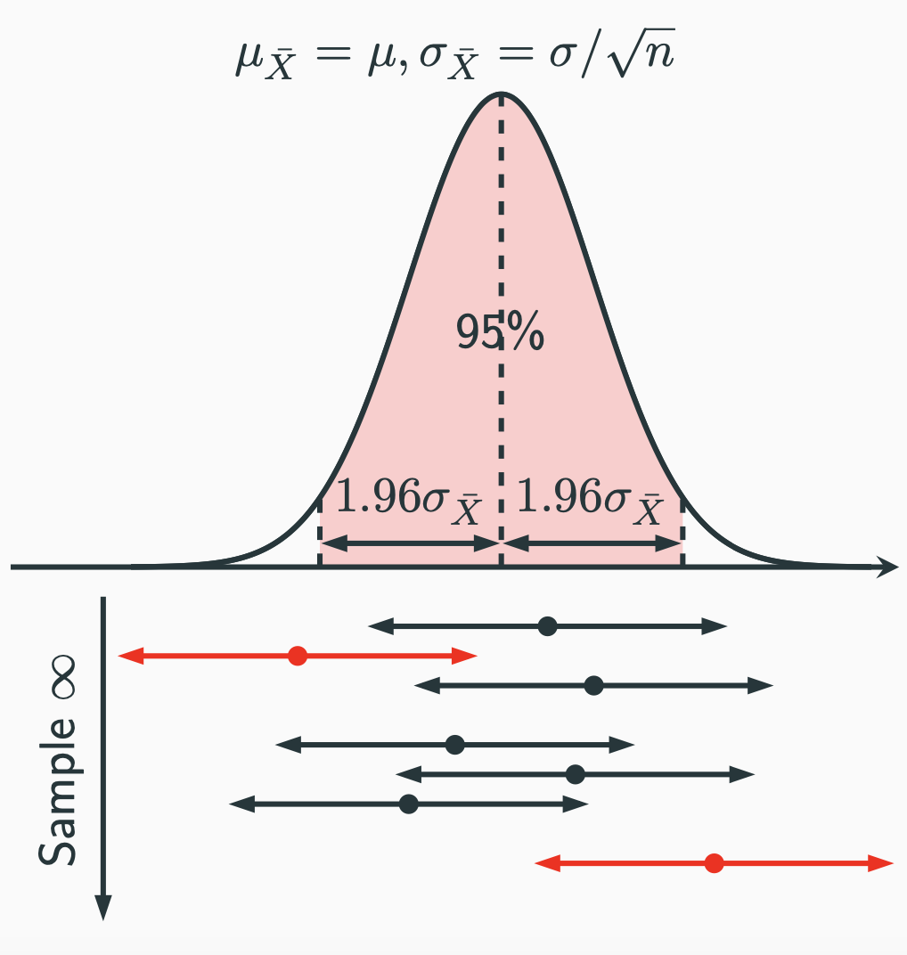
Again, we can think of probability as relative frequency. Whenever we draw a sample, we can put the values of $\bar{X}$, $n$ and $\sigma$ into the formula to get a 95% CI. Then we draw another sample. The value of $\bar{X}$ will change and we get another 95% CI. If we keep doing this for a large number of times, we will get a large number of different 95% CIs. Among all those 95% CIs, 95% of them will contain the population mean $\mu$. That’s exactly what the formula $(\mathrm{M})$ tells us. To help us visualise the interpretation, we can draw the sampling distribution of the sample mean:

Note that the width on the $x$-axis of the red-shaded area is $2 \times 1.96\sigma_{\bar{X}} = 3.92 \frac{\sigma}{\sqrt{n}}$, which is the same length as the 95% CI. Whenever we draw a sample, we have a sample mean represented by the dot at the bottom. Then we can construct a 95% CI with the length $3.92 \frac{\sigma}{\sqrt{n}}$ (double arrowed line) centred around the sample mean. Due the same length of the 95% CI and the bottom width of the red-shaded area, whenever a sample mean falls inside the red-shaded area, the 95% CI is guaranteed to cover the population mean (the middle dashed line). Whenever a sample mean falls outside the red-shaded area, the 95% CI is guaranteed NOT to cover the population mean. The probability of the sample mean falling into the red-shaded area is basically 95% due to the normal distribution.

This seems to be some convoluted interpretation of confidence interval at first, but if think about it, it does make sense. The interpretation is not only correct but strictly follows our frequentist definition of probability as well.

Confidence Interval For The Mean With Unknown Variance

In general, it is unrealistic for us to know the population variance $\sigma^2$ in practice. How can we construct a 95% confidence interval? Intuitively, we can just replace the population standard deviation $\sigma$ with the sample standard deviation $s=\sqrt{\frac{1}{n-1}\sum_{i=1}^n (x_i - \bar{x})^2}$, can we? It is natural for us to do that. Does this work? Here is the simulation from $100,000$ 95% confidence intervals constructed by drawing samples with size $n=8$ from a normal population with a known variance:

	By $\boldsymbol{\bar{x} \pm 1.96 \cfrac{\sigma}{\sqrt{n}}}$	By $\boldsymbol{\bar{x} \pm 1.96 \cfrac{s}{\sqrt{n}}}$
% of intervals covering $\mu$	$95.24\%$	$90.55\%$

By definition, we should expect about 95% of those 95% CIs containing the population mean $\mu$, and $\bar{x} \pm 1.96 \cfrac{\sigma}{\sqrt{n}}$ does. However, only ~90% of the 95% CIs by $\bar{x} \pm 1.96 \cfrac{s}{\sqrt{n}}$ contain $\mu$, indicating we have introduced some errors when we replace $\sigma$ with $s$.

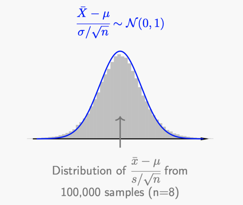
The reason we can construct 95% CIs as previously described is based on the property that $\cfrac{\bar{X}-\mu}{\sigma/\sqrt{n}} \sim \mathcal{N}(0,1)$. However, when we replace $\sigma$ with $s$, the random variable $\cfrac{\bar{X}-\mu}{S/\sqrt{n}}$ does not follow a standard normal distribution. Here is the histogram of from $100,000$ simulations compared with a standard normal curve:

As you can see, the distribution of $\cfrac{\bar{X}-\mu}{S/\sqrt{n}}$ (grey histogram) is a bit lower than the standard normal around $0$ and higher at the tail regions.

Student’s $t$-Distribution

In order to construct 95% CIs for the population mean without knowing the population variance, we need to figure out the distribution of $\cfrac{\bar{X}-\mu}{S/\sqrt{n}}$ if it exists.

How are we going to figure out the distribution of $\cfrac{\bar{X}-\mu}{S/\sqrt{n}}$? It looks difficult, but what we can do is to manipulate the expression to something we are familiar with. It may not solve the problem, but at least we might get some hints. For example, we know $\bar{X}$ is a normal random variable under certain conditions. We do not know the distribution of $S$, but we do know that the distribution of $S^2$ is related to the $\chi^2$ distribution. Therefore, we manipulate the numerator an denominator to that direction:

$$ \begin{aligned} \cfrac{\bar{X}-\mu}{S/\sqrt{n}} &= \cfrac{\sqrt{n}(\bar{X}-\mu)}{S} = \cfrac{\sqrt{n}(\bar{X}-\mu)}{\sqrt{S^2}} = \cfrac{\frac{\bar{X}-\mu}{\sigma/\sqrt{n}}}{\sqrt{S^2}/\sigma} = \cfrac{\frac{\bar{X}-\mu}{\sigma/\sqrt{n}}}{\sqrt{\frac{S^2}{\sigma^2}}} \\[15pt] &= \cfrac{\frac{\bar{X}-\mu}{\sigma/\sqrt{n}}}{\sqrt{\frac{(n-1)S^2}{\sigma^2} \cdot \frac{1}{n-1}}} \end{aligned} $$

Now both the numerator and the denominator have something we are familiar with. The numerator $\frac{\bar{X}-\mu}{\sigma/\sqrt{n}}$ is basically a standard normal random variable. The term $\frac{(n-1)S^2}{\sigma^2}$ in the denominator is a $\chi^2(n-1)$ random variable. From here, we can actually figure out the PDF of $\cfrac{\bar{X}-\mu}{S/\sqrt{n}}$, and we call this $\boldsymbol{t}$-distribution.

We are not going to do the derivation during the lecture, but I put it into the Extra Reading Material after the class. The $\boldsymbol{t}$-distribution was discovered by the English statistician William Gosset, who worked for Guinness Brewery when he figured out the distribution of $\cfrac{\bar{X}-\mu}{S/\sqrt{n}}$ and published under the pseudonym Student. Hence the name $t$-distribution.

The random variable $T$ is defined as:

$$T = \cfrac{Z}{\sqrt{U/\nu}}$$

where $Z$ is a standard normal random variable, $U$ is a $\chi^2$ random variable with a degree of freedom (DOF) $\nu$ (the Greek letter nu), and $Z$ and $U$ are independent. In this case, the random variable $T$ follows a $\boldsymbol{t}$-distribution with a degree of freedom of $\nu$ that comes from the $\chi^2$ random variable $U$. We write it as:

$$T \sim \boldsymbol{\mathcal{T}}(\nu)$$

Now we know that:

$$\cfrac{\bar{X}-\mu}{S/\sqrt{n}} \sim \boldsymbol{\mathcal{T}}(n-1)$$

Therefore, instead of using the normal distribution, we should use $\boldsymbol{t}$-distribution with a degree of freedom $n-1$ for the construction of 95% CIs for the population mean with an unknown variance.

Properties of The $\boldsymbol{t}$-Distributions

As you can see, the $\boldsymbol{t}$-distribution only has one parameter, that is, the degree of freedom $\nu$. From the Extra Reading Material, we know that the PDF of a $\boldsymbol{t}$-distribution is:

$$f_{T}(t) = \cfrac{\Gamma \left(\frac{\nu+1}{2}\right)}{\sqrt{\pi\nu}\,\Gamma \left(\frac{\nu}{2}\right)} \left( 1+\cfrac{t^2}{\nu} \right)^{-\frac{\nu+1}{2}} $$

where $\nu$ is the degree of freedom. That is a very scary PDF. Luckily, we do not really need to memorise it, but you do need to practice calculating related probabilities using R or Excel.

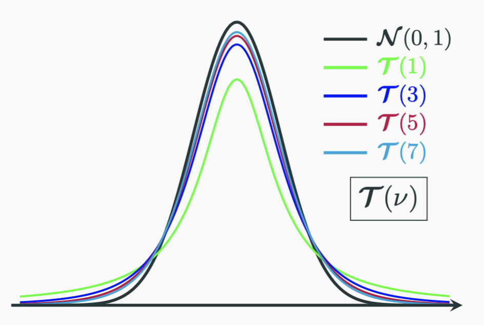
As you have already seen the simulation, the shape of a $\boldsymbol{t}$-distribution is very similar to a standard normal distribution. It is symmetrical around $0$, just a bit lower than the standard normal near $0$ and higher at the tail regions. With increasing $\nu$, the $\boldsymbol{t}$-distribution becomes more and more like the standard normal and eventually will become the standard normal when $\nu \to \infty$:

Use $\boldsymbol{t}$-Distributions To Construct 95% CIs For $\boldsymbol{\mu}$

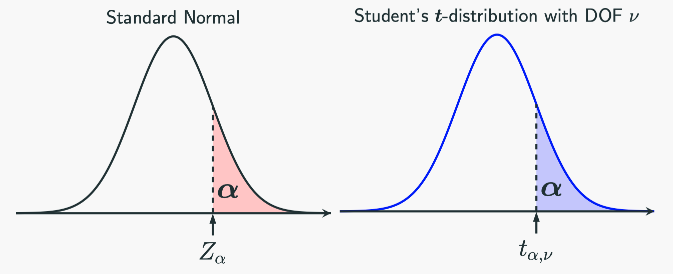
Let’s just introduce some new notations to make things easier to discuss. Visually, this is the notation:

In the standard normal distribution, we use $Z_{\alpha}$ to represent the value such that the probability of falling into the region greater than $Z_{\alpha}$ (upper tail region) is $\alpha$. That is:

$$\mathbb{P}(X \geqslant Z_{\alpha}) = \alpha \textmd{, where } X \sim \mathcal{N}(0,1)$$

Since the standard normal is symmetrical with respect to $0$, it is straightforward for us to see $Z_{\alpha} = -Z_{1-\alpha}$. For example, $Z_{0.025} = -Z_{0.975} \approx 1.96$.

Therefore, the 95% CI for the mean $\mu$ when we know $\sigma$ can be written as $\left[ \bar{X} - Z_{0.025} \frac{\sigma}{\sqrt{n}}, \bar{X} + Z_{0.025} \frac{\sigma}{\sqrt{n}} \right]$.

Similarly, we use $t_{\alpha,\nu}$ to denote the value in a $\boldsymbol{t}$-distribution with a degree of freedom $\nu$ such that the probability of falling to the region in greater than $t_{\alpha,\nu}$ (upper tail region) is $\alpha$:

$$\mathbb{P}(X \geqslant t_{\alpha,\nu}) = \alpha \textmd{, where } X \sim \boldsymbol{t}_\nu$$

Hence the 95% CI for the mean $\mu$ when we do not know $\sigma$ can be written as $\left[ \bar{X} - t_{0.025,n-1} \frac{s}{\sqrt{n}}, \bar{X} + t_{0.025,n-1} \frac{s}{\sqrt{n}} \right]$, where $s$ is the sample standard deviation and $n$ is the sample size. Actually, to construct a confidence interval with a confidence level of $(1-\alpha) \times 100\%$, we do:

$$\left[ \bar{X} - t_{\frac{\alpha}{2},n-1} \cfrac{S}{\sqrt{n}}, \bar{X} + t_{\frac{\alpha}{2},n-1} \cfrac{S}{\sqrt{n}} \right]$$

We are going to use those notations a lot even for other distributions such as $\chi^2$ and the future $\boldsymbol{F}$-distributions. The principle is exactly the same.

One-sided Confidence Interval

What we have been doing in the lecture is to construct a two-sided CI. That is, we compute both the lower and upper bounds. It is also useful to construct one-sided CIs. As the name suggest, we want an interval like $[a, \infty)$ or $(-\infty, b]$. This is left for you to finish in your homework.